041 GDAL: time series
Purpose
In this section, we'll continue to look at the MODIS LAI, with a view to forming a time series dataset. At the end of this session, you will be able to generate a 3D numpy array of some MODIS geophysical variable for a selcted area and time.
Prerequisites
You must make sure you can recall the details of the work covered in 040_GDAL_mosaicing_and_masking. You will also need to know how to do graph plotting, including sub-figures and errorbars, and image display.
Test
You should run a NASA account test if you have not already done so.
Introduction
Recall that we can use getModis from geog0111.modisUtils as a simple interface to download and stitch MODIS data.
For example:
from geog0111.modisUtils import getModis

warp_args = {
    'dstNodata'     : 255,
    'format'        : 'MEM',
    'cropToCutline' : True,
    'cutlineWhere'  : "FIPS='UK'",
    'cutlineDSName' : 'data/TM_WORLD_BORDERS-0.3.shp'
}

kwargs = {
    'tile'      :    ['h17v03','h18v03','h17v04','h18v04'],
    'product'   :    'MCD15A3H',
    'sds'       :    'Lai_500m',
    'doys'       : [1,5,41],
    'year'      : 2019,
    'warp_args' : warp_args
}

datafiles,bnames = getModis(verbose=False,timeout=10000,**kwargs)

print(datafiles)
print(bnames)
['work/stitch_Lai_500m_2019_001_Tiles_h17v03_h18v03_h17v04_h18v04_Selektor_FIPS_UK_warp.vrt', 'work/stitch_Lai_500m_2019_005_Tiles_h17v03_h18v03_h17v04_h18v04_Selektor_FIPS_UK_warp.vrt', 'work/stitch_Lai_500m_2019_041_Tiles_h17v03_h18v03_h17v04_h18v04_Selektor_FIPS_UK_warp.vrt']
['2019-001', '2019-005', '2019-041']
Timeseries
We can conveniently generate a timeseries dataset using the gdal VRT file approach we used in 040_GDAL_mosaicing_and_masking.
We can directly use the output from getModis for this.
We use gdal.BuildVRT() as we have previously, specifying the output name work/stitch_set.vrt here, and the list of SDS that goes in to the time series,datafiles here. The one difference is that we set separate=True for a time series (or for multiple bands) so the data aren't merged spatially.
from osgeo import gdal
import numpy as np

# build a VRT "work/stitch_set.vrt"
stitch_vrt = gdal.BuildVRT("work/stitch_set.vrt", datafiles,separate=True)
del stitch_vrt
# test it by reading and plotting
g = gdal.Open("work/stitch_set.vrt")

# apply scaling and read
data = g.ReadAsArray() * 0.1
print(data.shape,data.dtype)
(3, 2623, 1394) float64
The dataset is now 3D. The first dimensions represent the time samples, so:
data[0] -> bnames[0]
etc.
import numpy as np
for i in range(data.shape[0]):
    print(f'band {bnames[i]} -> mean {np.mean(data[i])}')
band 2019-001 -> mean 18.3917659748686
band 2019-005 -> mean 18.39242177274097
band 2019-041 -> mean 18.313179488806387
These are strange average LAI numbers. Why would that be?
Exercise 1
We have seen in 040_GDAL_mosaicing_and_masking that you can use gdal to creat a GeoTiff format image, for example with:
g = gdal.Warp(output_name, input_name ,format='GTiff',options=['COMPRESS=LZW'])
g.FlushCache()
- Convert the
gdalfilework/stitch_set.vrtto a more portable GeoTiff file calledwork/stitch_set.tif - Confirm that this has worked by reading and displaying data from the file
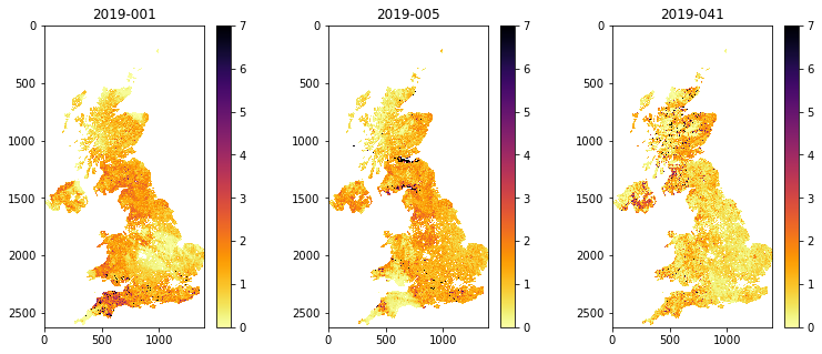
The reason for the 'funny' averages above was because the data is not masked: it includes invalid numbers (e.g. 255) where there are no data.
Now let's mask out invalid data points (> 10.0 when scaled by 0.1), and display the results:
# valid mask
data[data>10.0] = np.nan
print(data.shape)
(3, 2623, 1394)
from osgeo import gdal
import matplotlib.pyplot as plt

fig, axs = plt.subplots(1,3,figsize=(13,5))
axs = axs.flatten()

for i in range(data.shape[0]):
    im = axs[i].imshow(data[i],vmax=7,\
                cmap=plt.cm.inferno_r,interpolation='nearest')
    fig.colorbar(im, ax=axs[i])
    axs[i].set_title(bnames[i])
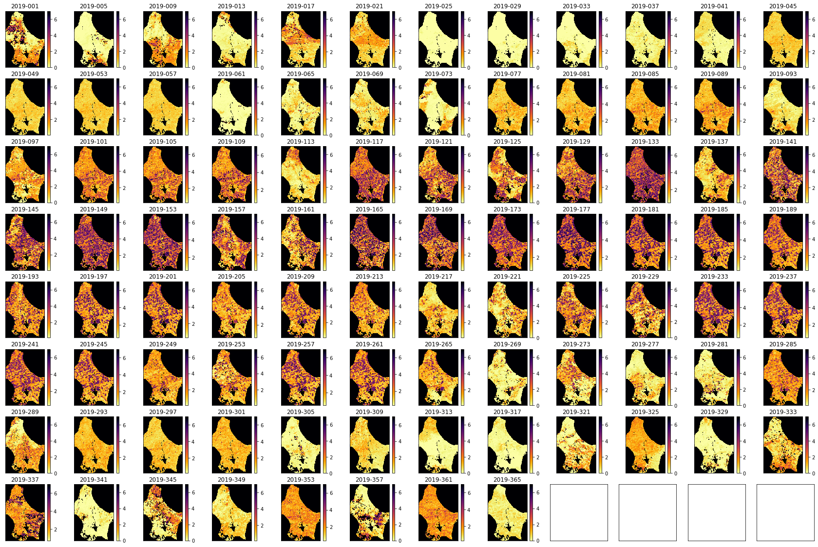
A year of data
To get a year of LAI data for Luxembourg, we can specify doys = [i for i in range(1,366,4)]. Note that we could have chosen any location, but we select a small country to make the running more feasible in a practical session.
If the data are already downloaded into the local cache, it should not take too long to form the time series. It will need to generate the VRT files for how every many files and tile you have requested, so that may take some tens of minutes, even if the HDF files are already generated.
If you are attempting to get data not already in the cache, it will take some considerable time to download these datasets for whole years, for multiple tiles.
If you want to download a dataset that is not covered in these notebooks, you are of course welcome to do so, but plan your work ahead of time, and try to pre-download the data before attempting any processing. In such a case, you should take some code such as that below and paste it into a Python file and run that as a Python script from a command line. You might make sure you set:
'verbose' : True
in the kwargs dictionary if you want some feedback about any long-running processes.
from geog0111.modisUtils import getModis

warp_args = {
    'dstNodata'     : 255,
    'format'        : 'MEM',
    'cropToCutline' : True,
    'cutlineWhere'  : "FIPS='LU'",
    'cutlineDSName' : 'data/TM_WORLD_BORDERS-0.3.shp'
}

kwargs = {
    'tile'      :    ['h18v03','h18v04'],
    'product'   :    'MCD15A3H',
    'sds'       :    'Lai_500m',
    'doys'      : np.arange(1,366,4),
    'year'      : 2019,
    'warp_args' : warp_args
}

datafiles,bnames = getModis(verbose=False,timeout=10000,**kwargs)
# check the files
print(f'filenames of the form: {datafiles[0]}\n')
print(bnames)
filenames of the form: work/stitch_Lai_500m_2019_001_Tiles_h18v03_h18v04_Selektor_FIPS_LU_warp.vrt

['2019-001', '2019-005', '2019-009', '2019-013', '2019-017', '2019-021', '2019-025', '2019-029', '2019-033', '2019-037', '2019-041', '2019-045', '2019-049', '2019-053', '2019-057', '2019-061', '2019-065', '2019-069', '2019-073', '2019-077', '2019-081', '2019-085', '2019-089', '2019-093', '2019-097', '2019-101', '2019-105', '2019-109', '2019-113', '2019-117', '2019-121', '2019-125', '2019-129', '2019-133', '2019-137', '2019-141', '2019-145', '2019-149', '2019-153', '2019-157', '2019-161', '2019-165', '2019-169', '2019-173', '2019-177', '2019-181', '2019-185', '2019-189', '2019-193', '2019-197', '2019-201', '2019-205', '2019-209', '2019-213', '2019-217', '2019-221', '2019-225', '2019-229', '2019-233', '2019-237', '2019-241', '2019-245', '2019-249', '2019-253', '2019-257', '2019-261', '2019-265', '2019-269', '2019-273', '2019-277', '2019-281', '2019-285', '2019-289', '2019-293', '2019-297', '2019-301', '2019-305', '2019-309', '2019-313', '2019-317', '2019-321', '2019-325', '2019-329', '2019-333', '2019-337', '2019-341', '2019-345', '2019-349', '2019-353', '2019-357', '2019-361', '2019-365']
We can build a VRT dataset as before:
stitch_vrt = gdal.BuildVRT("work/stitch_time.vrt", datafiles,separate=True)
del stitch_vrt
And read the data into a numpy array:
from osgeo import gdal

g = gdal.Open("work/stitch_time.vrt")
data = g.ReadAsArray() * 0.1
We can now plot the data on sub-plots:
import matplotlib.pyplot as plt

shape=(8,12)
x_size,y_size=(30,20)

fig, axs = plt.subplots(*shape,figsize=(x_size,y_size))
axs = axs.flatten()
plt.setp(axs, xticks=[], yticks=[])

for i in range(data.shape[0]):
    im = axs[i].imshow(data[i],vmax=7,cmap=plt.cm.inferno_r,\
                       interpolation='nearest')
    axs[i].set_title(bnames[i])
    fig.colorbar(im, ax=axs[i])
Plotting time series
We might now want to plot some time series. We will need to know the day of year associated with each spatial dataset in the time series. We could just attempt to specify doys = [i for i in range(1,366,4)] as above. But that might not be robust (e.g. if no data were available for some particular day).
It is better to try to develop an internally consistent dataset. The doy information associated with each spatial dataset in the time series is encoded in the band name strings we examined above, such as 2019-001.
First, extract the doy from bnames:
print(bnames)
['2019-001', '2019-005', '2019-009', '2019-013', '2019-017', '2019-021', '2019-025', '2019-029', '2019-033', '2019-037', '2019-041', '2019-045', '2019-049', '2019-053', '2019-057', '2019-061', '2019-065', '2019-069', '2019-073', '2019-077', '2019-081', '2019-085', '2019-089', '2019-093', '2019-097', '2019-101', '2019-105', '2019-109', '2019-113', '2019-117', '2019-121', '2019-125', '2019-129', '2019-133', '2019-137', '2019-141', '2019-145', '2019-149', '2019-153', '2019-157', '2019-161', '2019-165', '2019-169', '2019-173', '2019-177', '2019-181', '2019-185', '2019-189', '2019-193', '2019-197', '2019-201', '2019-205', '2019-209', '2019-213', '2019-217', '2019-221', '2019-225', '2019-229', '2019-233', '2019-237', '2019-241', '2019-245', '2019-249', '2019-253', '2019-257', '2019-261', '2019-265', '2019-269', '2019-273', '2019-277', '2019-281', '2019-285', '2019-289', '2019-293', '2019-297', '2019-301', '2019-305', '2019-309', '2019-313', '2019-317', '2019-321', '2019-325', '2019-329', '2019-333', '2019-337', '2019-341', '2019-345', '2019-349', '2019-353', '2019-357', '2019-361', '2019-365']
we can try to extract the information from these strings then. Let's build up to that, by considering a single example string, and work out how to deal with that. Once we know that, we can build a loop around it (e.g. in a list comprehension like we had for [i for i in range(1,366,4)].
# convert to 1 by splitting the string
test = '2019-001'
int(test.split('-')[1])
1
doy = [int(i.split('-')[1]) for i in bnames]
print(doy)
[1, 5, 9, 13, 17, 21, 25, 29, 33, 37, 41, 45, 49, 53, 57, 61, 65, 69, 73, 77, 81, 85, 89, 93, 97, 101, 105, 109, 113, 117, 121, 125, 129, 133, 137, 141, 145, 149, 153, 157, 161, 165, 169, 173, 177, 181, 185, 189, 193, 197, 201, 205, 209, 213, 217, 221, 225, 229, 233, 237, 241, 245, 249, 253, 257, 261, 265, 269, 273, 277, 281, 285, 289, 293, 297, 301, 305, 309, 313, 317, 321, 325, 329, 333, 337, 341, 345, 349, 353, 357, 361, 365]
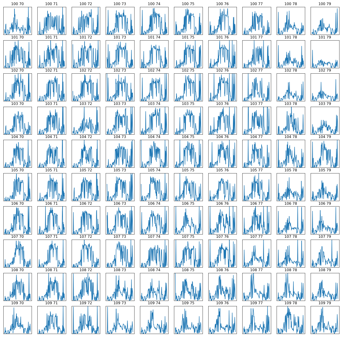
It is interesting to see a set of sub-plots for a range of pixel locations. We can follow tghe approach we have taken to sub-plots previously, but now we want to make use of the 2D nature of the sub-plot axs variable (recall that previously we have flattened this to a 1D representation).
We will define a sub-plot shape: shape=(10,10) and a starting pixel pixel = (100,70). We will then loop in row and column to produce the sub-plots:
import matplotlib.pyplot as plt

x_size,y_size=(20,20)

shape=(10,10)
fig, axs = plt.subplots(*shape,figsize=(x_size,y_size))
plt.setp(axs, xticks=[], yticks=[])

pixel = (100,70)
x = doy

for i in range(shape[0]):
    p0 = pixel[0] + i
    for j in range(shape[1]):
        p1 = pixel[1] + j
        im = axs[i,j].plot(x,data[:,p0,p1])
        axs[i,j].set_title(f'{p0} {p1}')
        # ensure the same scale for all
        axs[i,j].set_ylim(0,7)
Exercise 2
- Produce a set of spatial plots of the quantity
Fpar_500mover Luxembourg for 2019
Exercise 3
Write a function called modisAnnual(**kwargs) with arguments based on:
warp_args = {
    'dstNodata'     : 255,
    'format'        : 'MEM',
    'cropToCutline' : True,
    'cutlineWhere'  : "FIPS='LU'",
    'cutlineDSName' : 'data/TM_WORLD_BORDERS-0.3.shp'
}

kwargs = {
    'tile'      :    ['h18v03','h18v04'],
    'product'   :    'MCD15A3H',
    'sds'       :    ['Lai_500m', 'Fpar_500m'],
    'doys'      : np.arange(1,366,4),
    'year'      : 2019,
    'warp_args' : warp_args
    'ofile_root': 'work/output_filename_ex3'
}
where sds is a list of SDS
That returns:
bnames  : names for the items in first (time) dimension
odict   : a dictionary with items in sds for keys and the names of associated VRT files as values
Uncertainty and weighting
The full set of SDS available is
['Fpar_500m',
 'Lai_500m',
 'FparLai_QC',
 'FparExtra_QC',
 'FparStdDev_500m',
 'LaiStdDev_500m']
We should always examine any uncertainty information available when trying to interpret a dataset. In this exercise, we will take the uncertainty, defined as a standard deviation, and generate a weight from this in the form:
W = 1/(std * std)
where std is the uncertainty. Where this weighting is high, we can put more emphasis on the reliability of the data than when it is low.
We make modisAnnual() available from geog0111.modisUtils so we can load multiple SDS datasets into a data dictionary:
from geog0111.modisUtils import modisAnnual

warp_args = {
    'dstNodata'     : 255,
    'format'        : 'MEM',
    'cropToCutline' : True,
    'cutlineWhere'  : "FIPS='LU'",
    'cutlineDSName' : 'data/TM_WORLD_BORDERS-0.3.shp'
}

kwargs = {
    'tile'      :    ['h18v03','h18v04'],
    'product'   :    'MCD15A3H',
    'sds'       :    ['Fpar_500m','Lai_500m','FparLai_QC','FparExtra_QC','FparStdDev_500m','LaiStdDev_500m']
,
    'doys'      : np.arange(1,366,4),
    'year'      : 2019,
    'warp_args' : warp_args
}

# run
odict,bnames = modisAnnual(**kwargs)

# outputs
print(odict,bnames)
{'Fpar_500m': 'work/output_filename_Selektor_FIPS_LU_YEAR_2019_DOYS_1_365_SDS_Fpar_500m.vrt', 'Lai_500m': 'work/output_filename_Selektor_FIPS_LU_YEAR_2019_DOYS_1_365_SDS_Lai_500m.vrt', 'FparLai_QC': 'work/output_filename_Selektor_FIPS_LU_YEAR_2019_DOYS_1_365_SDS_FparLai_QC.vrt', 'FparExtra_QC': 'work/output_filename_Selektor_FIPS_LU_YEAR_2019_DOYS_1_365_SDS_FparExtra_QC.vrt', 'FparStdDev_500m': 'work/output_filename_Selektor_FIPS_LU_YEAR_2019_DOYS_1_365_SDS_FparStdDev_500m.vrt', 'LaiStdDev_500m': 'work/output_filename_Selektor_FIPS_LU_YEAR_2019_DOYS_1_365_SDS_LaiStdDev_500m.vrt'} ['2019-001', '2019-005', '2019-009', '2019-013', '2019-017', '2019-021', '2019-025', '2019-029', '2019-033', '2019-037', '2019-041', '2019-045', '2019-049', '2019-053', '2019-057', '2019-061', '2019-065', '2019-069', '2019-073', '2019-077', '2019-081', '2019-085', '2019-089', '2019-093', '2019-097', '2019-101', '2019-105', '2019-109', '2019-113', '2019-117', '2019-121', '2019-125', '2019-129', '2019-133', '2019-137', '2019-141', '2019-145', '2019-149', '2019-153', '2019-157', '2019-161', '2019-165', '2019-169', '2019-173', '2019-177', '2019-181', '2019-185', '2019-189', '2019-193', '2019-197', '2019-201', '2019-205', '2019-209', '2019-213', '2019-217', '2019-221', '2019-225', '2019-229', '2019-233', '2019-237', '2019-241', '2019-245', '2019-249', '2019-253', '2019-257', '2019-261', '2019-265', '2019-269', '2019-273', '2019-277', '2019-281', '2019-285', '2019-289', '2019-293', '2019-297', '2019-301', '2019-305', '2019-309', '2019-313', '2019-317', '2019-321', '2019-325', '2019-329', '2019-333', '2019-337', '2019-341', '2019-345', '2019-349', '2019-353', '2019-357', '2019-361', '2019-365']
We can read some of these data in now:
from osgeo import gdal

g = gdal.Open(odict['Lai_500m'])
if g:
    Lai_500m = g.ReadAsArray() * 0.1
    print(Lai_500m.shape)

g = gdal.Open(odict['LaiStdDev_500m'])
if g:
    LaiStdDev_500m = g.ReadAsArray() * 0.1
    print(LaiStdDev_500m.shape)
(92, 175, 122)
(92, 175, 122)
There is a feature in the LaiStdDev_500m dataset where some pixels have apparently zero uncertainty. Indeed, all LAI values with an uncertainty under 1.0 seem suspect as individual values. So we treat them hear, to set all values less than 1 to 1.
We know that LAI values over 10 (100 * 0.1) are invalid, so we should make sure these are also weighted zero:
import numpy as np

weight = np.zeros_like(LaiStdDev_500m)
std = LaiStdDev_500m

# fix low values
std[std<1.0] = 1.0

mask = (std > 0)
weight[mask] = 1./(std[mask]**2)

weight[Lai_500m > 10] = 0.
weight[LaiStdDev_500m==0] = 0.
# look at some stats
print(weight.min(),weight.max())
0.0 1.0
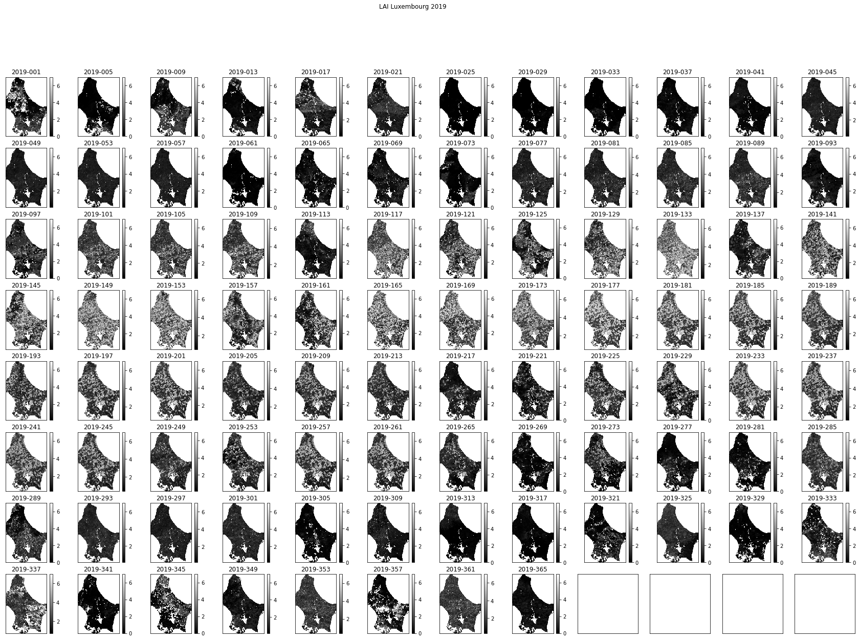
We can now go ahead and plot the dataset and the weights. We switch to a greyscale colourmap to make the interpretation of numbers easier.
# produce image plots of the both quantities
import matplotlib.pyplot as plt

shape=(8,12)
x_size,y_size=(30,20)

fig, axs = plt.subplots(*shape,figsize=(x_size,y_size))
axs = axs.flatten()
plt.setp(axs, xticks=[], yticks=[])
fig.suptitle("LAI Luxembourg 2019")
for i in range(Lai_500m.shape[0]):
    im = axs[i].imshow(Lai_500m[i],vmax=7,cmap=plt.cm.gray,\
                       interpolation='nearest')
    axs[i].set_title(bnames[i])
    fig.colorbar(im, ax=axs[i])
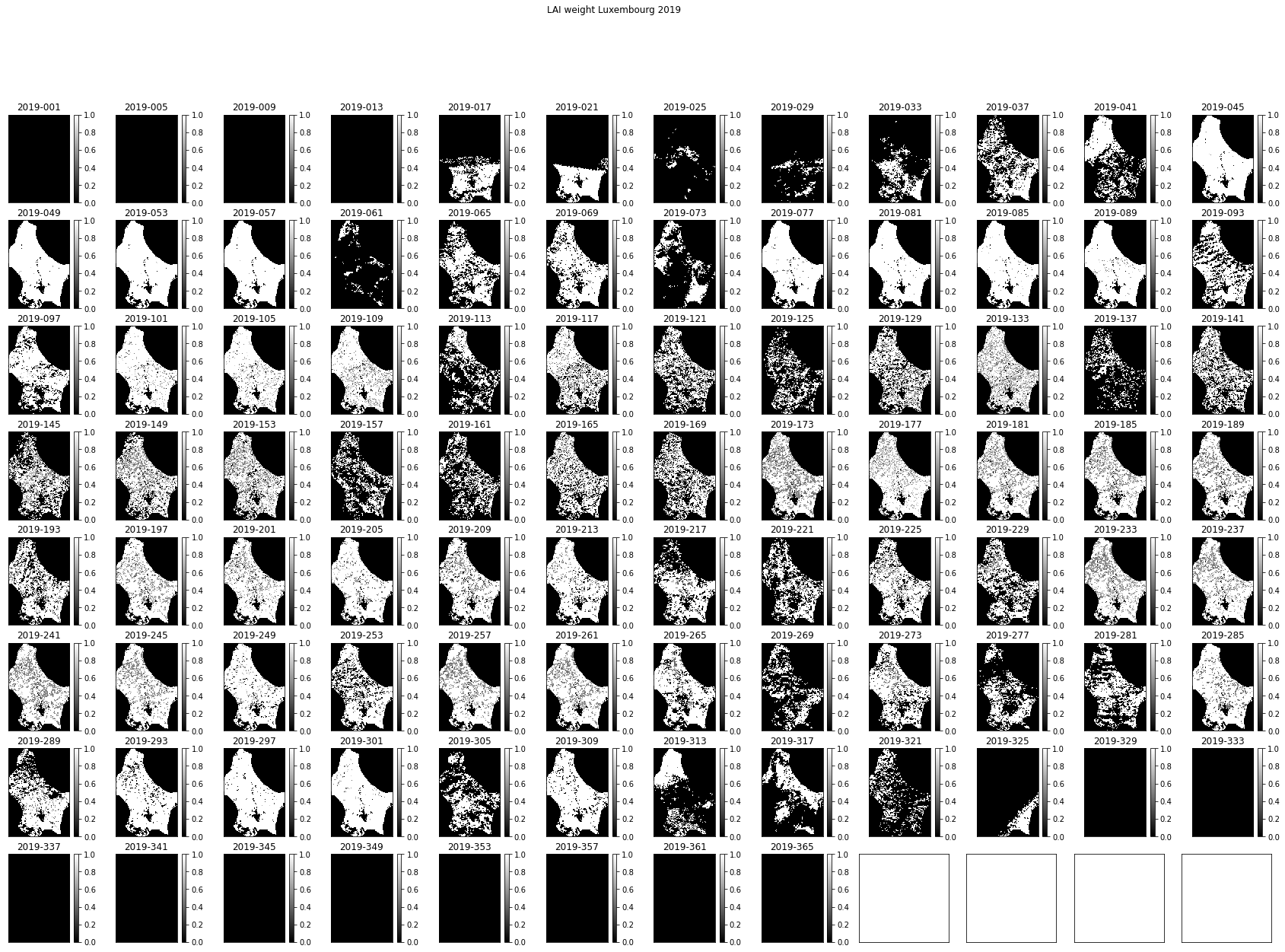
# Plot the weight
import matplotlib.pyplot as plt

shape=(8,12)
x_size,y_size=(30,20)

fig, axs = plt.subplots(*shape,figsize=(x_size,y_size))
axs = axs.flatten()
plt.setp(axs, xticks=[], yticks=[])
fig.suptitle("LAI weight Luxembourg 2019")

for i in range(Lai_500m.shape[0]):
    im = axs[i].imshow(weight[i],vmax=1,cmap=plt.cm.gray,\
                       interpolation='nearest')
    axs[i].set_title(bnames[i])
    fig.colorbar(im, ax=axs[i])
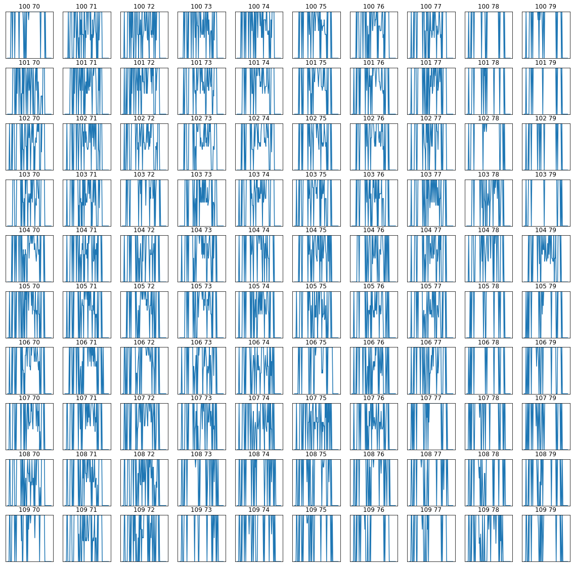
# LAI time series
import matplotlib.pyplot as plt

doy = [int(i.split('-')[1]) for i in bnames]

x_size,y_size=(20,20)

shape=(10,10)
fig, axs = plt.subplots(*shape,figsize=(x_size,y_size))
plt.setp(axs, xticks=[], yticks=[])

pixel = (100,70)
x = doy

for i in range(shape[0]):
    p0 = pixel[0] + i
    for j in range(shape[1]):
        p1 = pixel[1] + j
        im = axs[i,j].plot(x,Lai_500m[:,p0,p1])
        axs[i,j].set_title(f'{p0} {p1}')
        # ensure the same scale for all
        axs[i,j].set_ylim(0,7)

# weight time series plots
import matplotlib.pyplot as plt
doy = [int(i.split('-')[1]) for i in bnames]

x_size,y_size=(20,20)

shape=(10,10)
fig, axs = plt.subplots(*shape,figsize=(x_size,y_size))
plt.setp(axs, xticks=[], yticks=[])

pixel = (100,70)
x = doy

for i in range(shape[0]):
    p0 = pixel[0] + i
    for j in range(shape[1]):
        p1 = pixel[1] + j
        im = axs[i,j].plot(x,weight[:,p0,p1])
        axs[i,j].set_title(f'{p0} {p1}')
        # ensure the same scale for all
        axs[i,j].set_ylim(0,1)
We can look at an individual plot now, and use the weights for error bars.
In this case, we want to convert the array weight to an array error, applying the opposite of what we did above to get standard deviation, and multiplying by 1.96.
We want to avoid the division 1/0, so we first build an array the same as weight, but fiulled with zero values:
error = np.zeros_like(weight)
and then only do the division for the mask weight>0:
error[weight>0] = np.sqrt(1./(weight[weight>0] )) * 1.96
import matplotlib.pyplot as plt

error = np.zeros_like(weight)
error[weight>0] = np.sqrt(1./(weight[weight>0] )) * 1.96

doy = [int(i.split('-')[1]) for i in bnames]
p0,p1 = (107,72)
x_size,y_size=(10,5)

shape=(10,10)
fig, axs = plt.subplots(1,1,figsize=(x_size,y_size))

pixel = (100,70)
x = doy

axs.errorbar(x,Lai_500m[:,p0,p1],yerr=error[:,p0,p1])
axs.set_title(f'{p0} {p1}')
# ensure the same scale for all
axs.set_ylim(0,7)
axs.set_xlabel('DOY 2019')
axs.set_ylabel('LAI')
Text(0, 0.5, 'LAI')
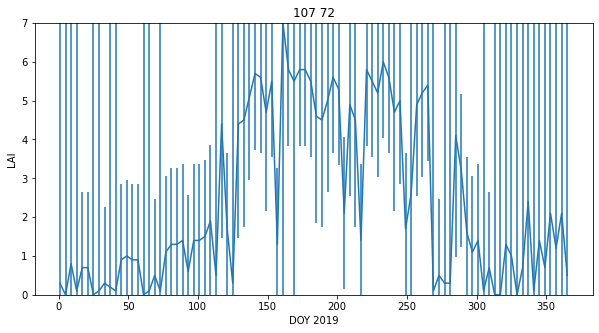
We might question the validity of some of the LAI uncertainty here: we expect LAI to have a smnooth trajectory in time, but that is clearly not always the case here. However, they provide a traceable estimate of the reliability of each individual measurement and are useful in that respect.
Exercise 3
- Write a function
getLaithat takes as argument:year : integer year tile : list of tiles to process fips : country fips code (e.g. BE for Belgium)
and returns the annual LAI, standard deviation and day of year
- test your code for Belgium for 2018 for tiles
['h17v03','h18v03','h17v04','h18v04'] - show the shape of the arrays returned
Hint: You may find it useful to use modisAnnual
Summary
We now know how to combine geospatial data in both space and time VRT files using gdal. Remember that we can also do such things using numpy, but if we are able to keep the geospatial information and other metadata in a gdal file, so much the better. We have seen how to write the dataset to a portable file format such as GeoTiff.
We have seen that some datasets such as the MODIS LAI product come with a per-pixel estimate of uncertainty. We have investigated this data field and used it to provide a weighting to associate with the reliability of each pixel. We have seen how to generate, filter, and process 3D spatio-temporal datasets. The examples here
Remember:
from geog0111.modisUtils import modisAnnual
help(modisAnnual)
We have also seen how we can incrementally develop codes to do more complex tasks and wrap up a utility such as getLai in the exercise above to retrieve a ready-to-use dataset.