024 Image display

Purpose

We have seen from 020_Python_files and 021_URLs how to access both text and binary datasets, either from the local file system or from a URL and in 023 Plotting how to use matplotlib for plotting graphs.

In this section, we will learn how to view images using matplotlib.

You might follow these notes up by looking at the Python package folium for interactive displays.

Prerequisites

You will need some understanding of the following:

001 Using Notebooks
002 Unix with a good familiarity with the UNIX commands we have been through.
003 Getting help
010 Variables, comments and print()
011 Data types
012 String formatting
013_Python_string_methods
020_Python_files
021_URLs
022_Pandas
023 Plotting

Test

You should run a NASA account test if you have not already done so.

Read and plot a dataset

MODIS

We have seen in 021_URLs how we can access a MODIS dataset. In an exercise we wrote a function getModisTiledata that returned a dictionary of spatial datasets, given a MODIS HDF filename. Here, we will use the similar function modis.get_data that returns the same form of data dictionary, but driven by the year and day of year (doy). The product and other parameters are specified in the keyword arguments. We will look into MODIS products in more detail in a subsequent session. In this session, we will use MCD15A3H and

For example, to get the LAI product MCD15A3H and the land cover product MCD12Q1, layer LC_Type1 to visualise. Many of these datasets are pre-cached for you, so you should get a fast response. If the plotting seems to be taking too long, set verbose=True in the kwargs to get details of the underlying processing.

First then, we access the product MCD15A3H. This is produced every 4 days in a year, so in specifying doy, we use doy=4*n + 1 for the nth dataset of the year.

from  geog0111.modisUtils import getModisTiledata

kwargs = {
    'product'    : 'MCD15A3H',
    'tile'       : 'h17v03',
    'year'       : 2019,
    'doy'        : 41
}
data_MCD15A3H = getModisTiledata(verbose=False,timeout=300,**kwargs)
# specify day of year (DOY) and year
print(*data_MCD15A3H.keys())

Fpar_500m Lai_500m FparLai_QC FparExtra_QC FparStdDev_500m LaiStdDev_500m

# loop over dictionary items
for k,v in data_MCD15A3H.items():
    # do some neat formatting on k
    print(f'{k:<20s}: {v.shape}')

Fpar_500m           : (2400, 2400)
Lai_500m            : (2400, 2400)
FparLai_QC          : (2400, 2400)
FparExtra_QC        : (2400, 2400)
FparStdDev_500m     : (2400, 2400)
LaiStdDev_500m      : (2400, 2400)

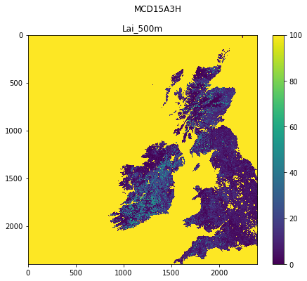
So any of these datasets, data[Fpar_500m], data[Lai_500m] are two dimensional datasets ((2400, 2400)) that we might display as images. For example data[Lai_500m].

We follow much the same recipe as for plotting line graphs, but instead of using axs.plot() we use axs.imshow(). Further, we can set the subplot title with axs.set_title(k) as before. We can usefully include a colour wedge with the plot with fig.colorbar(im, ax=axs).

When we plot with axs.imshow(), we can optionally use the keywords vmin= and vmax= to set upper and lower thresholds for the data plotted.

You should generally use interpolation='nearest' when plotting an image dataset as a measurement (e.g. a remote sensing dataset), otherwise it may be interpolated.

import matplotlib.pyplot as plt

k = 'Lai_500m'
name = f'{kwargs["product"]}'

# plot size 
x_size,y_size = 8,6
shape = (1,1)

fig, axs = plt.subplots(shape[0],shape[1],figsize=(x_size,y_size))
# dont flatten if shape is (1,1)
if shape[0] == 1 and shape[1] == 1:  
    axs = [axs]
else:
    axs = axs.flatten()
# set the figure title
fig.suptitle(name)

# plot image data: use vmin and vmax to set limits
im = axs[0].imshow(data_MCD15A3H[k],\
                   vmin=0,vmax=100,\
                   interpolation='nearest')
axs[0].set_title(k)
fig.colorbar(im, ax=axs[0])

<matplotlib.colorbar.Colorbar at 0x7fc61f3f9bd0>

png

Exercise 1

Plot the first datasets in data_MCD15A3H as subplots in a 2 x 2 shape.

Hint: Use a loop for the keys of data_MCD15A3H. Set up the 2 x 2 subplots with:

fig, axs = plt.subplots(2,2,figsize=(x_size,y_size))
axs = axs.flatten()

then you can refer to the subplot axes as ax[0], ax[1], ax[2] and ax[3] when you loop over the keys. Don't forget to increase x_size,y_size appropriately.

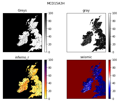
Colourmaps

As you would expect, you can customise your plots. We illustrate this by changing the colourmap used here in a pseudocolour display of the data. For some others, please see the matplotlib tutorial.

There are various ways to set the colour map, but when working with sub-images, trhe easiest is of the form:

im = ax.imshow(data)
im.set_cmap(c)

where c here is some colourmap.

For further discussions on colourmaps and options see the relevant tutorial and the colour map reference.

In this set of sub-plots, we switch off the image ticks for a clearer plot.

import matplotlib.pyplot as plt

k = 'Lai_500m'
name = f'{kwargs["product"]}'

# plot size 
x_size,y_size = 8,6
shape = (2,2)

fig, axs = plt.subplots(*shape,figsize=(x_size,y_size))
# dont flatten if shape is (1,1)
if shape[0] == 1 and shape[1] == 1:  
    axs = [axs]
else:
    axs = axs.flatten()

# this new cmd switches off the tick
plt.setp(axs, xticks=[], yticks=[])

# set the figure title
fig.suptitle(name)

cmaps = ['Greys','gray','inferno_r','seismic']

for i,c in enumerate(cmaps):
    # plot image data
    im = axs[i].imshow(data_MCD15A3H[k],\
                   vmin=0,vmax=100,\
                   interpolation='nearest')
    im.set_cmap(c)
    axs[i].set_title(c)
    fig.colorbar(im, ax=axs[i])

png

Exercise 2

write a function called im_display that takes as input:
- a data dictionary
- a list of keywords of datasets to plot
- optionally:
  - a title
  - a colourmap name
  - lower and upper limits for plot data (vmin, vmax)
  - x_size,y_size
  - subplots shape : e.g. (2,2)

You should assume some default values for the optional items if not given. For the subplots shape, assume it is (n,1) where n is the length of the keyword list.

You should set the default values of vmin and vmax to None, as this just then takes the dataset default minimum and maximum.

Your code should be well-documented.

test your code

Note that you will have to experiment a bit with the x_size,y_size values to get a good plot. It is not easy to automate that.

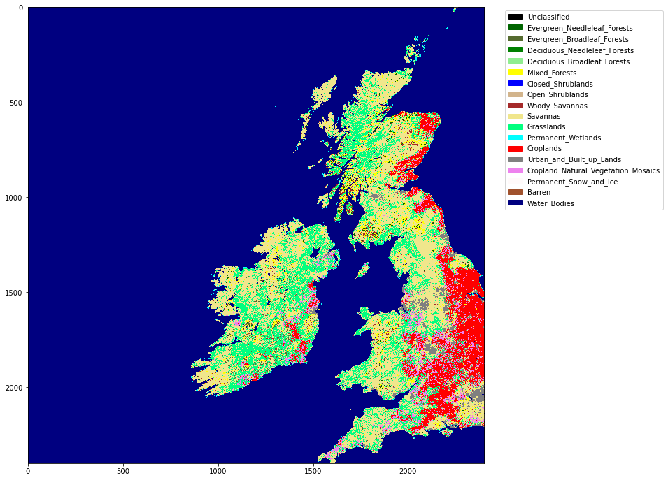
Quantised data: Land Cover

Sometimes we want quantised colourmaps, for example for a land cover classification map. You can do these perfectly well in matplotlib, but the process is a little more involved.

We will take as an example the MODIS product MCD12Q1 over the UK. The land cover layer we are interested in is called LC_Type1. The land cover names associated with this are given in the file data/LC_Type1_colour.csv, along with example colour mappings.

import pandas as pd

lc_Type1 = pd.read_csv('data/LC_Type1_colour.csv')
lc_Type1

	code	class	colour
0	-1	Unclassified	black
1	1	Evergreen_Needleleaf_Forests	darkgreen
2	2	Evergreen_Broadleaf_Forests	darkolivegreen
3	3	Deciduous_Needleleaf_Forests	green
4	4	Deciduous_Broadleaf_Forests	lightgreen
5	5	Mixed_Forests	yellow
6	6	Closed_Shrublands	blue
7	7	Open_Shrublands	tan
8	8	Woody_Savannas	brown
9	9	Savannas	khaki
10	10	Grasslands	springgreen
11	11	Permanent_Wetlands	cyan
12	12	Croplands	red
13	13	Urban_and_Built_up_Lands	grey
14	14	Cropland_Natural_Vegetation_Mosaics	violet
15	15	Permanent_Snow_and_Ice	snow
16	16	Barren	sienna
17	17	Water_Bodies	navy

The process of setting up a colourmap is explained in this Earth Lab page.

The three steps are:

* set up colour names associated with the class names
* generate matplotlib cmap and norm objects from these
* set up the legend

We can choose colour names from the matplotlib gallery if we don't like the defaults set up.

It is an annual dataset, with only valid files for January 1st of the year.

from  geog0111.modisUtils import getModisTiledata

kwargs = {
    'product'    : 'MCD12Q1',
    'tile'       : 'h17v03',
    'year'       : 2019,
    'doy'        : 1
}

data_MCD12Q1 = getModisTiledata(verbose=False,timeout=300,**kwargs)

# generate matplotlib cmap and norm objects from these
import matplotlib

cmap = matplotlib.colors.\
        ListedColormap(list(lc_Type1['colour']))
norm = matplotlib.colors.\
        BoundaryNorm(list(lc_Type1['code']), len(lc_Type1['code']))

import matplotlib.patches
# set up the legend
legend_labels = dict(zip(list(lc_Type1['colour']),list(lc_Type1['class'])))
patches = [matplotlib.patches.Patch(color=c, label=l)
           for c,l in legend_labels.items()]

# plot
import matplotlib.pyplot as plt
x_size,y_size = 12,12
fig, axs = plt.subplots(1,figsize=(x_size,y_size))
im = axs.imshow(data_MCD12Q1['LC_Type1'],cmap=cmap,norm=norm,interpolation='nearest')
plt.legend(handles=patches,
          bbox_to_anchor=(1.4, 1),
          facecolor="white")

<matplotlib.legend.Legend at 0x7fc60c2f0c90>

png

Exercise 3

Write a function called plot_lc that takes as input modis land cover dataset and plots the associated land cover map
You might use x_size,y_size as optional inputs to improve scaling
Show the function operating

Summary

In this section, we have learned how to plot images from datasets we have read in or downloaded from the web. We have concentrated on MODIS datasets, stored in a data dictionary. We used modis.get_data to load the MODIS datasets. We developed a function called im_display to provide a simple wrapper for plotting.

We have also looked into how to do categorised mapping, for example for land cover, and written a function called plot_lc to achieve this.

Remember:

        import matplotlib
        import matplotlib.pyplot as plt

function	comment	keywords
`im = axs.imshow(data2D)`	Display image of 2D data array `data2D` on sub-plot axis `axs` and return display object `im`	`vmin=` : minimum threshold for image display
		`vmax=` : maximum threshold for image display
		`interpolation=` : interpolation style (e.g. `'nearest'`
`fig.colorbar(im)`	Set colour bar for image plot object `im`	`ax=axs` plot on sub-plot `axs`
`im.set_cmap(c)`	set colourmap `c` for image object `im`
	Examples being `['Greys','gray','inferno_r','seismic']`
`cmap = matplotlib.colors.ListedColormap(list_of_colours)`	set `cmap` to `Colormap` object from list of colours `list_of_colours`
`norm = matplotlib.colors.BoundaryNorm(list, nbound)`	set `BoundaryNorm` object `norm` to boundaries of values from `list` with `nbound` values
`matplotlib.patches.Patch(color=c, label=l)`	Set patches for legend with colours from list `c` and labedl from list `l`
`plt.legend(handles=patches)`	set figure legend using `patches`	`bbox_to_anchor=(1.4, 1)` : shift of legend
		`facecolor="white"` : facecolourt of legend (white here)

We have also used getModisTiledata from geog0111.modisUtils:

help(getModisTiledata)

Help on function getModisTiledata in module geog0111.modisUtils:

getModisTiledata(doy=None, year=2020, month=1, day=1, tile='h08v06', product='MCD15A3H', timeout=None, sds='None', version='006', no_cache=False, cache=None, verbose=False, force=False, altcache='/shared/groups/jrole001/geog0111')
    return MODIS data dictionary of given SDS for given MODIS tile

    N.B. You need to have a username and password to access the data.
    These are available at https://urs.earthdata.nasa.gov

    Example of use:

      from geog0111.modisUtils import getModisdata

      modinfo = {
        'product'  : 'MCD15A3H',
        'year'     : 2020,
        'month'    : 1,
        'day'      : 5,
        'tile'     : 'h08v06'
      }

      data = getModisdata(**modinfo,verbose=False)
      print(f'-> {*data.keys()}')

      -> Fpar_500m Lai_500m FparLai_QC FparExtra_QC FparStdDev_500m LaiStdDev_500m


    Returns data read from MODIS data product file
              e.g. what you would find on

           https://e4ftl01.cr.usgs.gov/MOTA/MCD15A3H.006/2020.01.05/MCD15A3H.A2020005.h08v06.006.2020010210940.hdf

              Downloaded to some cache location e.g.

              /Users/plewis/.modis_cache/e4ftl01.cr.usgs.gov/MOTA/MCD15A3H.006/2020.01.05/MCD15A3H.A2020005.h08v06.006.2020010210940.hdf

    Control options:
      year : int of year (2000+ for Terra, 2002+ for Aqua products)
             (year=2020)

      doy  : day of year (doy=None)
      OR
      month: int of month (1-12) (month=1)
      day  : int of day (1-31, as appropriate) (day=1)

      tile    : string of tile (tile='h08v06')  
      product : string of MODIS product name (product='MCD15A3H')
      version : int or string of version (version='006')
      sds     : only load these SDS (string or list)

      timeout : timeout in seconds
      verbose : verbosity (verbose=False)


    Cache options:
      no_cache : Set True if you don't want to use the cache 
                 (no_cache=False)

                 This is common for most functions, but 
                 modisFile() will use a cache in any case, 
                 as it has to store the file somewhere. 
                 If you don;'t want to keep that, then 
                 you can delete after use.
      cache    : Use cache='/home/somewhere/else' to specify 
                 a personal cache location with write permission 
                 (ie somewhere in your filespace)
                 Specify personal cache root. By default, 
                 this will be ~, and the cache will go into 
                 ~/.modis_cache. You can change that to 
                 somewhere else
                 here. It will still use the sub-directory 
                 .modis_cache.
                 Use cache='/home/somewhere/else' to specify a 
                 personal cache location with write permission 
                 (ie somewhere in your filespace)
      altcache : Specify system cache root. 
                 Use altcache='/home/notme/somewhere' to specify a 
                 system cache location with read permission 
                 (ie somewhere not necessarily in your filespace)
      force    : Bool : Use force=True to override information in the cache

    Get the URL associated with a MODIS product
    for a certain date and version. Since this can
    involve  an expensive call to get the html to access the file URL
    The html data used can be cached unless no_cache = True
    (See modisHTML())

    This function returns the URL for the product/date page listing

    The caching is done to avoid repeated calls to expensive URL downloads.
    The idea is that there will be a system cache, where shared files will
    be set up (where you have read permission), and a personal cache
    where you can read and write your own files. Unless you
    use force=True or disble cache with no_cache=True, then the code
    will look in (i) personal; (ii) system cache before attempting
    to download any file from a URL.

    The cached files are stored in the same structure as the URL, i.e

    https://e4ftl01.cr.usgs.gov/MOTA/MCD15A3H.006/2020.01.05/MCD15A3H.A2020005.h08v06.006.2020010210940.hdf

    will be stored (personal cache) as:

    ~/.modis_cache/e4ftl01.cr.usgs.gov/MOTA/MCD15A3H.006/2020.01.05/MCD15A3H.A2020005.h08v06.006.2020010210940.hdf

    The html cache is what is returned from e.g.

    https://e4ftl01.cr.usgs.gov/MOTA/MCD15A3H.006/2020.01.05

    and is stored as eg

    ~/.modis_cache/e4ftl01.cr.usgs.gov/MOTA/MCD15A3H.006/2020.01.05/index.html

Last update: December 6, 2022